
from: https://towardsdatascience.com/progan-how-nvidia-generated-images-of-unprecedented-quality-51c98ec2cbd2
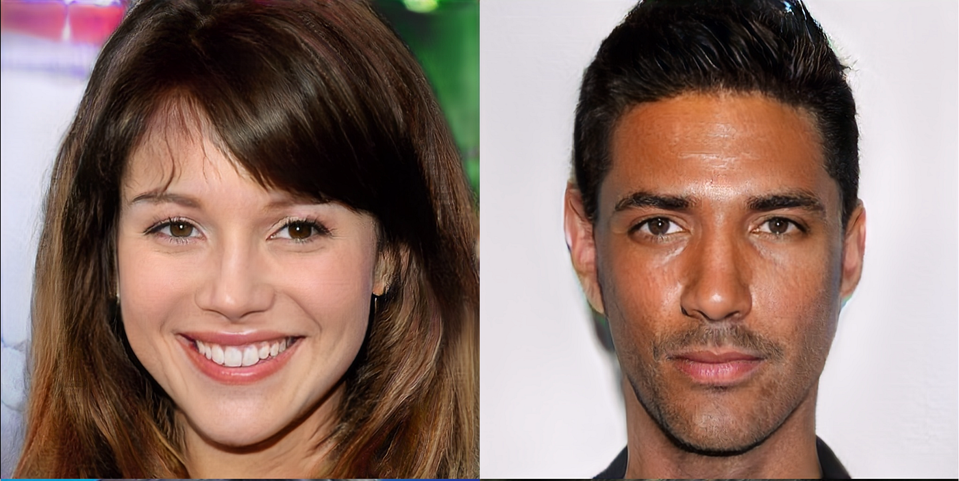
The people in the high resolution images above may look real, but they are actually not — they were synthesized by a ProGAN trained on millions of celebrity images. “ProGAN” is the colloquial term for a type of generative adversarial network that was pioneered at NVIDIA. It was published by Karras et al. last year in Progressive Growing of GANs For Improved Quality, Stability, and and Variation. In this post, we are going to walk through this paper to understand how this type of network works, how it can produce images like the ones above, and why this was a breakthrough.
This post assumes you are familiar with deep learning for visual tasks in general, but not that you have extensive knowledge of GANs.
A Brief History of GANs
A New Kind of Generative Model
Generative Adversarial Networks (GANs) have been around for a few years now. They were introduced in a now famous 2014 paper by Ian Goodfellow and colleagues at the University of Montreal, and have been a popular field of inquiry ever since.
In short, GANs are a type of generative model that attempts to synthesize novel data that is indistinguishable from the training data. This is a form of unsupervised learning. It has two neural networks, locked in competition: a generator, that is fed a vector of random numbers and outputs synthesized data, and a discriminator, which is fed a piece of data and outputs a probability of it being from the training set (as opposed to synthesized). In other words, the generator creates “fakes”, and the discriminator attempts to distinguish these “fake” samples from the “real” ones.
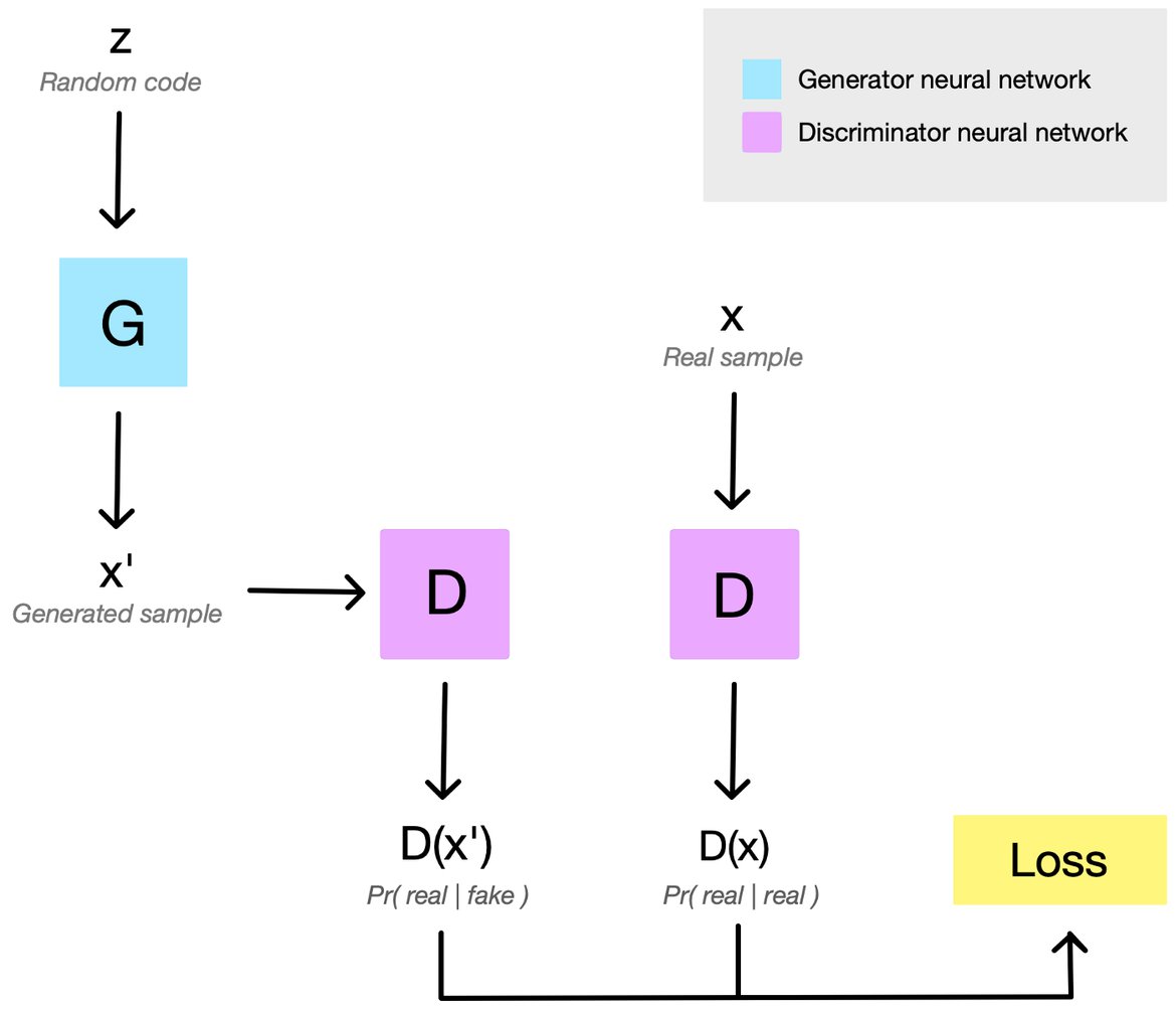
Both networks start out performing quite poorly at their tasks, but when training goes well, they improve in tandem until the generator is producing convincing fakes. The two networks are locked in a zero sum game, where the success of one corresponds to a failure of the other. Because of this, the value of the loss function at any given time does not tell us how well-trained the system is overall, only how well the generator or discriminator are doing relative to the other.
The random code we feed into the generator is particularly important. It is a source of noise that enables the synthesized samples to be new and unique. It also tends to control the output in interesting ways. As we linearly interpolate around the vector space of the random code, the corresponding generated output also interpolates smoothly, sometimes even in ways that are intuitive for us humans.
Challenges and Limitations
While this was all very exciting for researchers interested in new ways to learn representations of unlabeled data, using GANs in practice was often quite difficult. From the beginning, practitioners noticed that they were challenging to train. This is largely due to a problem called mode collapse. Mode collapse can occur when the discriminator essentially “wins” the game, and the training gradients for the generator become less and less useful. This can happen relatively quickly during training, and when it does, the generator starts outputting nearly the same sample every time. It stops getting better.
Even Ian Goodfellow admits he got lucky when the hyperparameters he chose for his first GAN worked when he tried it on a hunch— they could have easily failed. In the years since, the research community has come up with many ways to make training more reliable. Certain families of architectures seem to work better than others, and several variations on the adversarial loss functions have been explored. Some of these seem more stable than others. I’d recommend Are GANs Created Equal? A Large Scale Study by Lucic et al., an excellent recent review of the GAN landscape, if you’d like to read more.
However, none of these approaches have eliminated the issue entirely, and the theoretical reasons for mode collapse remain an area of active research.
Generating Images
A major improvement in image generation occured in 2016, when Radford et al published Unsupervised Representation Learning With Deep Convolutional Generative Adversarial Networks. They had found a family of GAN architectures that worked well for creating images, called “DCGANs” for short. DCGANs got rid of the pooling layers used in some CNNs, and relied on convolutions and transpose convolutions to change the representation size. Most layers were followed by a batch normalization and a leaky ReLU activation.
Yet even DCGANs could only create images of a certain size. The higher the resolution of an image, the easier it becomes for the discriminator to tell the “real” images from the “fakes”. This makes mode collapse more likely. While synthesizing 32x32 or even 128x128 images became routine tutorial material, generating images at resolutions above 512x512 remained challenging in practice.
I should note, some image-to-image translation techniques can handle high resolutions, but that is a different task, since those only learn to change surface-level features of an input image, and are not generating an entirely new image from scratch.
As you might imagine, the difficulty of generating large images from scratch severely limited the usefulness of GANs for many kinds of practical applications.
Toward Higher Image Resolutions
It was in this context that the team at NVIDIA presented the stunningly detailed 1024x1024 images at the top of this article, generated by their new ProGAN. Better yet, they knew of no reason their technique could not be used to synthesize even higher resolution images. It was even more efficient (in terms of training time) than previous GANs.
Growing GANs
Instead of attempting to train all layers of the generator and discriminator at once — as is normally done — the team gradually grew their GAN, one layer at a time, to handle progressively higher resolution versions of the images.

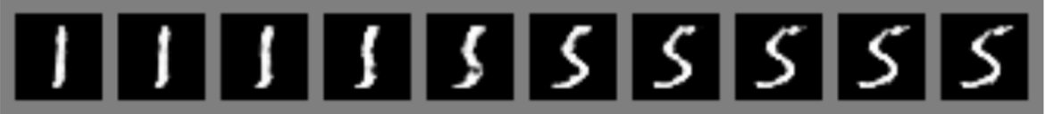
The ProGAN starts out generating very low resolution images. When training stabilizes, a new layer is added and the resolution is doubled. This continues until the output reaches the desired resolution. By progressively growing the networks in this fashion, high-level structure is learned first, and training is stabilized. source
To do this, they first artificially shrunk their training images to a very small starting resolution (only 4x4 pixels). They created a generator with just a few layers to synthesize images at this low resolution, and a corresponding discriminator of mirrored architecture. Because these networks were so small, they trained relatively quickly, and learned only the large-scale structures visible in the heavily blurred images.
When the first layers completed training, they then add another layer to G and D, doubling the output resolution to 8x8. The trained weights in the earlier layers were kept, but not locked, and the new layer was faded in gradually to help stabilize the transition (more on that later). Training resumed until the GAN was once again synthesizing convincing images, this time at the new 8x8 resolution.
In this way, they continued to add layers, double the resolution and train until the desired output size was reached.
The Effectiveness of Growing GANs
By increasing the resolution gradually, we are continuously asking the networks to learn a much simpler piece of the overall problem. The incremental learning process greatly stabilizes training. This, in combination with some training details we’ll discuss below, reduces the chance of mode collapse.
The low-to-high resolution trend also forces the progressively grown networks to focus on high level structure first (patterns discernible in the most blurred versions of the image), and fill in the details later. This improves the quality of the final image by reducing the likelihood that the network will get some high-level structure drastically wrong.
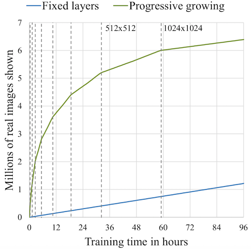
Increasing the network size gradually is also more computationally efficient than the more traditional approach of initializing all the layers at once. Fewer layers are faster to train, as there are simply fewer parameters in them. Since all but the final set of training iterations are done with a subset of the eventual layers, this leads to some impressive efficiency gains. Karras et al. found that their ProGAN generally trained about 2–6 times faster than a corresponding traditional GAN, depending on the output resolution.
The Architecture
In addition to gradually growing the networks, the authors of the NVIDIA paper made several other architectural changes to facilitate stable, efficient training.
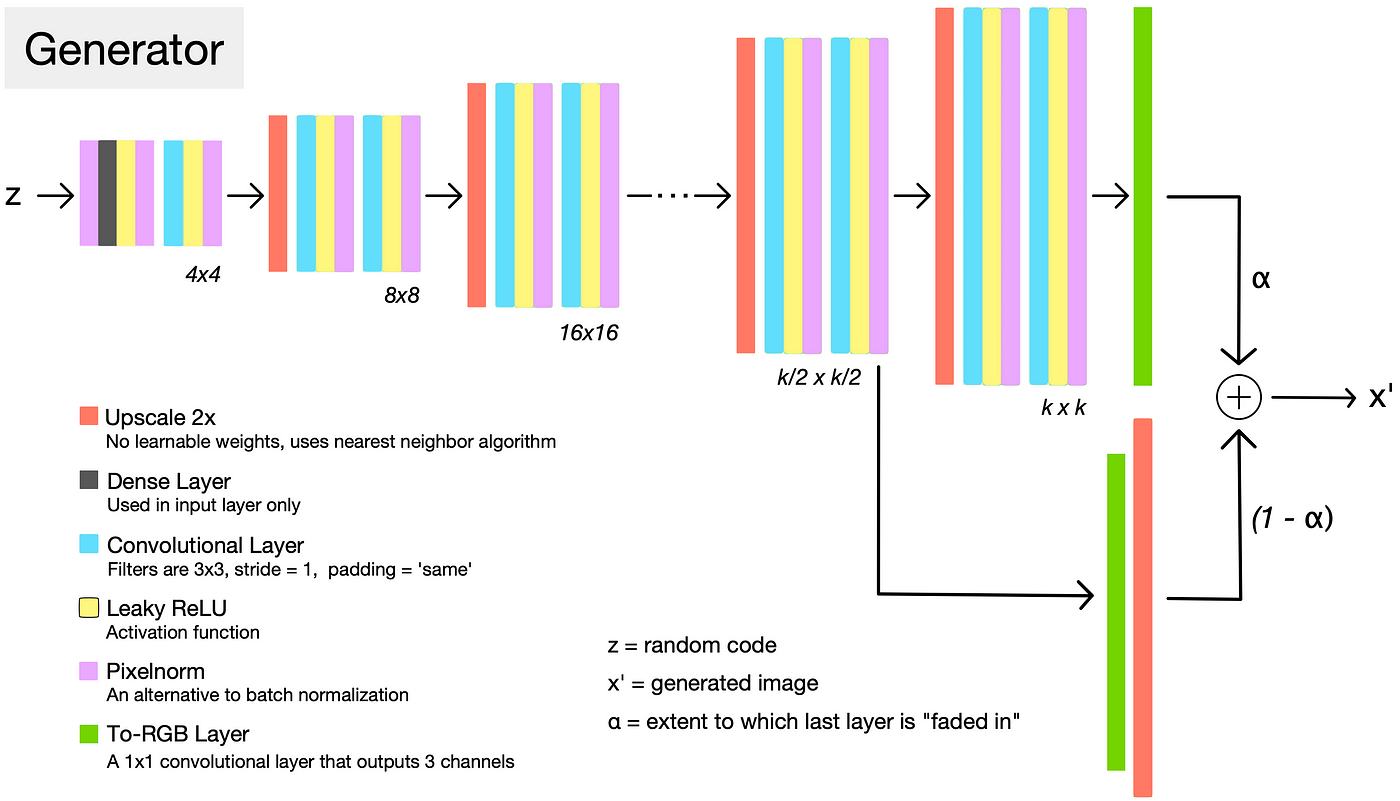
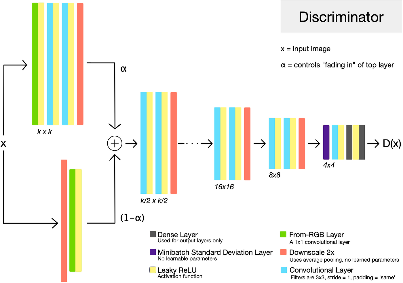
The generator architecture for a given resolution k follows a familiar high level pattern: each set of layers doubles the representation size, and halves the number of channels, until the output layer creates an image with just three channels corresponding to RGB. The discriminator does almost exactly the opposite, halving the representation size and doubling the number of channels with each set of layers. In both networks, the channel-doubling pattern is interrupted by capping the number of filters at a reasonable value, like 512, to prevent the total number of parameters from becoming too high.
In this sense, ProGAN resembles earlier image-producing GANs. A similar structure was used by DCGAN.
However, DCGAN used transpose convolutions to change the representation size. In constrast, ProGAN uses nearest neighbors for upscaling and average pooling for downscaling. These are simple operations with no learned parameters. They are then followed by two convolutional layers.
“Fading in” New Layers
The networks are progressively grown by adding a new set of layers to double the resolution each time training completes at the existing resolution. When new layers are added, the parameters in the previous layers remain trainable.
To prevent shocks in the pre-existing lower layers from the sudden addition of a new top layer, the top layer is linearly “faded in”. This fading in is controlled by a parameter α, which is linearly interpolated from 0 to 1 over the course of many training iterations. As you can see in the diagram above, the final generated image is the weighted sum of the last and second-to-last layers in the generator.
Pixel Normalization
Instead of using batch normalization, as is commonly done, the authors used pixel normalization. This “pixelnorm” layer has no trainable weights. It normalizes the feature vector in each pixel to unit length, and is applied after the convolutional layers in the generator. This is done to prevent signal magnitudes from spiraling out of control during training.

The Discriminator
The generator and discriminator are roughly mirror images of each other, and always grow in synchrony. The discriminator takes an input image x, which is either the output of the generator, or a training image scaled down to the current training resolution. As is typical of GAN discriminators, it attempts to distinguish the “real” training set images from the “fake” generated images. It outputs D(x), a value that captures the discriminator’s confidence that the input image came from the training set.
Minibatch Standard Deviation
In general, GANs tend to produce samples with less variation than that found in the training set. One approach to combat this is to have the discriminator compute statistics across the batch, and use this information to help distinguish the “real” training data batches from the “fake” generated batches. This encourages the generator to produce more variety, such that statistics computed across a generated batch more closely resemble those from a training data batch.
In ProGAN, this is done by inserting a “minibatch standard deviation” layer near the end of the discriminator. This layer has no trainable parameters. <mark>It computes the standard deviations of the feature map pixels across the batch, and appends them as an extra channel.</mark>
Equalized Learning Rate
The authors found that to ensure healthy competition between the generator and discriminator, it is essential that layers learn at a similar speed. To achieve this equalized learning rate, they scale the weights of a layer according to how many weights that layer has. They do this using the same formula as is used in He initialization, except they do it in every forward pass during training, rather than just at initialization.

Due to this intervention, no fancy tricks are needed for weight initialization — simply initializing weights with a standard normal distribution works fine.
The Loss Function
The authors say that the choice of loss function is orthogonal to their contribution — meaning that none of the above improvements rely on a specific loss function. It would be reasonable to use any of the popular GAN loss functions that have come out in the last few years.
However, if you are looking to follow the paper exactly, they used the improved Wasserstein loss function, also known as WGAN-GP. It is one of the fancier common loss functions, and has been shown to stabilize training and improve the odds of convergence.
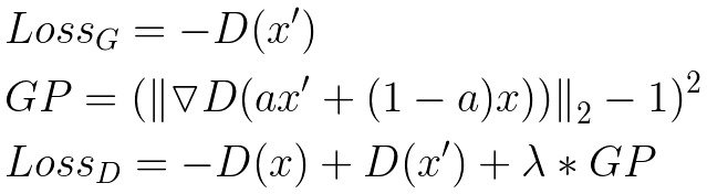
It is important to note that the WGAN-GP loss function expects D(x) and D(x’) to be unbounded real-valued numbers. In other words, the output of the discriminator is not expected to be a value between 0 and 1. This is slightly different than the traditional GAN formulation, which views the output of the discriminator as a probability.
Results
If you’ve made it this far, congrats! You now have a pretty good understanding of one of the most state-of-the-art image generation algorithms out there. If you would like to see more training details, there is an excellent official implementation that was released by the NVIDIA team. They also have a talk on the subject.
Thanks for reading! I hope this was a useful overview. Please leave a comment if you have questions, corrections, or suggestions for improving this post.
